Tangens hyperbolicus und Kotangens hyperbolicus
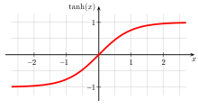
Tangens hyperbolicus und Kotangens hyperbolicus sind Hyperbelfunktionen. Man nennt sie auch Hyperbeltangens oder hyperbolischen Tangens bzw. Hyperbelkotangens oder hyperbolischen Kotangens.
Schreibweisen
| Tangens hyperbolicus: | 
|
| Kotangens hyperbolicus: | 
|
Definitionen


Hierbei bezeichnen  und
und  den Sinus
hyperbolicus bzw. Kosinus
hyperbolicus.
den Sinus
hyperbolicus bzw. Kosinus
hyperbolicus.
Eigenschaften
| Tangens hyperbolicus | Kotangens hyperbolicus | |
|---|---|---|
| Definitionsbereich | 
|
;

|
| Wertebereich | 
|
 ; ;

|
| Periodizität | keine | keine |
| Monotonie | streng monoton steigend |  streng monoton fallend
 streng monoton fallend
 |
| Symmetrien | Punktsymmetrie zum Koordinatenursprung | Punktsymmetrie zum Koordinatenursprung |
| Asymptoten |  
|
|
| Nullstellen | 
|
keine |
| Sprungstellen | keine | keine |
| Polstellen | keine |
|
| Extrema | keine | keine |
| Wendepunkte | 
|
keine |
Spezielle Werte
Der Kotangens hyperbolicus hat zwei Fixpunkte, d.h., es gibt zwei  ,
sodass
,
sodass
 .
.
Sie liegen bei  (Folge
 ![]() A085984 in
OEIS)
A085984 in
OEIS)
Umkehrfunktionen
Der Tangens hyperbolicus ist eine Bijektion  .
Die Umkehrfunktion
nennt man Areatangens
hyperbolicus. Sie ist für Zahlen x aus dem Intervall
.
Die Umkehrfunktion
nennt man Areatangens
hyperbolicus. Sie ist für Zahlen x aus dem Intervall  definiert und nimmt als Wert alle reellen Zahlen an. Sie lässt sich durch den
natürlichen Logarithmus
ausdrücken:
definiert und nimmt als Wert alle reellen Zahlen an. Sie lässt sich durch den
natürlichen Logarithmus
ausdrücken:

Für die Umkehrung des Kotangens hyperbolicus gilt:

Ableitungen


Die  -te
Ableitung ist gegeben durch
-te
Ableitung ist gegeben durch

mit den Euler-Zahlen An,k.
Additionstheorem
Es gilt das Additionstheorem

analog dazu:

Integrale


Weitere Darstellungen
Reihenentwicklungen
![\tanh x=\operatorname{sgn} x\left[1+\sum \limits _{{k=1}}^{\infty }(-1)^{k}\,2\,{\mathrm {e}}^{{-2k|x|}}\right]](/svg/77a679a8aa241b5c335498931b8199483e4d84e1.svg)

Der Anfang der Taylorreihe des Tangens hyperbolicus lautet:

Die  sind die Bernoulli-Zahlen.
Der Konvergenzradius
dieser Reihe ist
sind die Bernoulli-Zahlen.
Der Konvergenzradius
dieser Reihe ist  .
.
Kettenbruchdarstellung
Johann Heinrich Lambert zeigte folgende Formel:

Numerische Berechnung
Grundsätzlich kann der Tangens hyperbolicus über die bekannte Formel

berechnet werden, wenn die Exponentialfunktion  zur Verfügung steht. Es gibt jedoch folgende Probleme:
- Große positive Operanden lösen einen Überlauf aus, obwohl das Endergebnis immer darstellbar ist
- Für Operanden nahe an 0 kommt es zu einer numerischen Auslöschung, womit das Ergebnis ungenau wird
Fall 1:  ist eine große positive Zahl mit
  :
:
 ,
,
- wobei
 die Anzahl der signifikanten Dezimalziffern des verwendeten Zahlentyps ist,
was zum Beispiel beim 64-Bit-Gleitkommatyp double 16 ist.
die Anzahl der signifikanten Dezimalziffern des verwendeten Zahlentyps ist,
was zum Beispiel beim 64-Bit-Gleitkommatyp double 16 ist.
Fall 2:
ist eine kleine negative Zahl mit  :
:

Fall 3:
ist nahe an 0, z. B. für  :
:

-
lässt sich hier über die Taylorreihe
 sehr genau berechnen.
Fall 4: Alle übrigen :
Differentialgleichung
 löst folgende Differentialgleichungen:
 oder
oder

mit  und
und 
Komplexe Argumente


Anwendungen in der Physik
- Tangens und Kotangens hyperbolicus können benutzt werden, um die zeitliche
Abhängigkeit der Geschwindigkeit
beim Fall
mit Luftwiderstand oder auch beim Wurf nach unten zu beschreiben, wenn für
den Strömungswiderstand
eine turbulente
Strömung angesetzt wird (Newton-Reibung).
Das Koordinatensystem werde so gelegt, dass die Ortsachse nach oben zeigt. Für
die Geschwindigkeit gilt dann eine Differenzialgleichung der Form
 mit der Schwerebeschleunigung
g und einer Konstanten k > 0 mit der Einheit 1/m. Es gibt
dann immer eine Grenzgeschwindigkeit
mit der Schwerebeschleunigung
g und einer Konstanten k > 0 mit der Einheit 1/m. Es gibt
dann immer eine Grenzgeschwindigkeit  ,
die für
,
die für  erreicht wird, und es gilt:
- beim Fall oder Wurf nach unten mit einer Anfangsgeschwindigkeit kleiner
der Grenzgeschwindigkeit:
 mit
mit 
- beim Wurf nach unten mit einer Anfangsgeschwindigkeit größer der
Grenzgeschwindigkeit:
 mit
mit 
- beim Fall oder Wurf nach unten mit einer Anfangsgeschwindigkeit kleiner
der Grenzgeschwindigkeit:
- In der Speziellen
Relativitätstheorie ist der Zusammenhang zwischen Geschwindigkeit v
und Rapidität
 gegeben durch
  mit der Lichtgeschwindigkeit
c.
mit der Lichtgeschwindigkeit
c.
- Der Tangens hyperbolicus beschreibt ferner die thermische Besetzung eines
Zwei-Zustands-Systems in der Quantenmechanik:
Ist n die gesamte Besetzung der beiden Zustände und E ihr Energie-Unterschied, so
ergibt sich für die Differenz der Besetzungszahlen
 ,
wobei
,
wobei  die Boltzmann-Konstante
und T die absolute
Temperatur ist.
die Boltzmann-Konstante
und T die absolute
Temperatur ist.
- Wichtig für die Beschreibung der Magnetisierung eines Paramagneten ist die Brillouin-Funktion:
![B_{J}(x)={\frac {1}{J}}\left[\left(J+{\frac {1}{2}}\right)\coth \left(J\,x+{\frac {x}{2}}\right)-{\frac {1}{2}}\coth {\frac {x}{2}}\right]](/svg/908e314179a7227dfef7fc0313ae6a9da8801494.svg)
- Der Kotangens hyperbolicus tritt auch in der Kosmologie
auf: Die zeitliche Entwicklung des Hubble-Parameters
in einem flachen Universum, das im Wesentlichen nur Materie und Dunkle Energie enthält
(was ein gutes Modell für unser tatsächliches Universum ist), wird beschrieben
durch
 ,
wobei
,
wobei  eine charakteristische Zeitskala ist und
  der Grenzwert des Hubble-Parameters für
ist (
der Grenzwert des Hubble-Parameters für
ist ( ist dabei der heutige Wert des Hubble-Parameters,
  der Dichteparameter
für die Dunkle Energie). (Dieses Ergebnis ergibt sich leicht aus dem
zeitlichen Verhalten des Skalenparameters, das aus den Friedmann-Gleichungen
abgeleitet werden kann.) Bei der Zeitabhängigkeit des Dichteparameters der
Dunklen Energie tritt dagegen der Tangens hyperbolicus auf:
der Dichteparameter
für die Dunkle Energie). (Dieses Ergebnis ergibt sich leicht aus dem
zeitlichen Verhalten des Skalenparameters, das aus den Friedmann-Gleichungen
abgeleitet werden kann.) Bei der Zeitabhängigkeit des Dichteparameters der
Dunklen Energie tritt dagegen der Tangens hyperbolicus auf:  .
.


© biancahoegel.de
Datum der letzten Änderung: Jena, den: 14.11. 2025