Laguerre-Polynome
Laguerre-Polynome (benannt nach Edmond
Laguerre) sind spezielle Polynome,
die auf dem Intervall ![[0,\infty ]](/svg/52088d5605716e18068a460dec118214954a68e9.svg) ein orthogonales
Funktionensystem bilden. Sie sind die Lösungen der laguerreschen
Differentialgleichung. Eine wichtige Rolle spielen die Laguerre-Polynome in
der theoretischen
Physik, insbesondere in der Quantenmechanik.
ein orthogonales
Funktionensystem bilden. Sie sind die Lösungen der laguerreschen
Differentialgleichung. Eine wichtige Rolle spielen die Laguerre-Polynome in
der theoretischen
Physik, insbesondere in der Quantenmechanik.
Differentialgleichung und Polynome
Laguerresche Differentialgleichung
Die laguerresche Differentialgleichung
 ,
,
ist eine gewöhnliche lineare Differentialgleichung zweiter Ordnung für  und
und 
Sie ist ein Spezialfall der Sturm-Liouville-Differentialgleichung

Erste Polynome
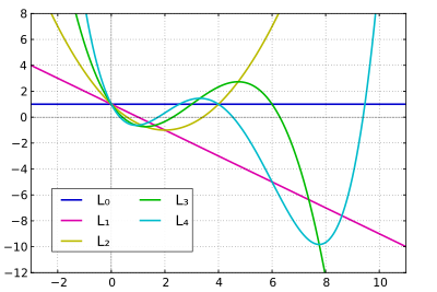
Die ersten fünf Laguerre-Polynome lauten

In der Physik wird üblicherweise eine Definition verwendet, nach der die
Laguerre-Polynome um einen Faktor  größer sind.
Eigenschaften
Rekursionsformeln
Das Laguerre-Polynom  lässt sich mit den ersten beiden Polynomen


über die folgende Rekursionsformel berechnen

Des Weiteren gelten folgende Rekursionsformeln:
 ,
, ,
, .
.
Eine explizite Formel für die Laguerre-Polynome lautet
 .
.
- Beispiel
Es wird das Polynom  für
für  berechnet. Also
 .
.
Um dieses Polynom zu erhalten, ist es notwendig, das Polynom  für
für  zu bestimmen. Es ergibt sich

Somit lautet das Polynom

Rodrigues-Formel
Das  -te
Laguerre-Polynom lässt sich mit der Rodrigues-Formel
wie folgt darstellen
-te
Laguerre-Polynom lässt sich mit der Rodrigues-Formel
wie folgt darstellen

und

Aus der ersten Gleichung berechnet sich das Laguerre-Polynom mit der Produktregel
für höhere Ableitungen und den Identitäten  ,
,
 sowie
sowie  gemäß
gemäß

Aus der zweiten Gleichung ergibt sich das Laguerre-Polynom mit dem binomischen
Lehrsatz und der Identität  wie folgt

Orthogonale Polynome
Da die Laguerre-Polynome für  und/oder
  divergent sind, bilden sie keinen Prähilbertraum
und keinen Hilbertraum.
Deshalb wird eine Gewichtsfunktion eingeführt welche die Lösung der
Differentialgleichung ungeändert lässt und welche dafür sorgt, dass die
Laguerre-Polynome quadratintegrierbar
werden. Unter diesen Voraussetzungen bilden die Eigenfunktionen
divergent sind, bilden sie keinen Prähilbertraum
und keinen Hilbertraum.
Deshalb wird eine Gewichtsfunktion eingeführt welche die Lösung der
Differentialgleichung ungeändert lässt und welche dafür sorgt, dass die
Laguerre-Polynome quadratintegrierbar
werden. Unter diesen Voraussetzungen bilden die Eigenfunktionen  eine Orthonormalbasis
im Hilbertraum
eine Orthonormalbasis
im Hilbertraum ![{\displaystyle L^{2}([0,\infty ],w(x)\mathrm {d} x)}](/svg/619373e228c51e399e63fe05b27c8b1e64e40dfe.svg) der quadratintegrierbaren Funktionen mit der Gewichtsfunktion
der quadratintegrierbaren Funktionen mit der Gewichtsfunktion  .
Demzufolge gilt
.
Demzufolge gilt

Hierbei bedeutet  das Kronecker-Delta.
- Beweis
Teil 1: Zunächst wird gezeigt, dass die Laguerre-Polynome mit dem
Gewicht
orthogonal sind, für  gilt demnach
Mit dem Sturm-Liouville-Operator  ergeben sich für die Laguerre-Polynome
  folgende Ausgangsgleichungen:
- (1)

und
- (2)
 .
.
Wird Gleichung (1) von links mit  multipliziert und von Gleichung (2), welche ebenfalls von links mit
multipliziert wird, subtrahiert, so ergeben sich die beiden Gleichungen:
multipliziert und von Gleichung (2), welche ebenfalls von links mit
multipliziert wird, subtrahiert, so ergeben sich die beiden Gleichungen:
- (3)

und
- (4)
 .
.
Zunächst wird Gleichung (3) zusammengefasst. Mit der Produktregel
für Ableitungen, der Term  bleibt hierbei unberücksichtigt, ergeben sich folgende Darstellungen

und
 .
.
Auf diese Weise wird erkennbar, dass der zweite Term in beiden Ableitungen gleich ist und bei der Differenzenbildung verschwindet, also:
- (5)

wobei  die Wronski-Determinante
der Funktionen
bedeutet.
die Wronski-Determinante
der Funktionen
bedeutet.
Zur Berechnung der Wronski-Determinante mittels der Abelschen
Identität wird die Differentialgleichung
 oder
oder  betrachtet, so dass eine hebbare
Singularität bei
betrachtet, so dass eine hebbare
Singularität bei  entsteht. Die Koeffizientenmatrix des Fundamentalsystems
lautet dann
entsteht. Die Koeffizientenmatrix des Fundamentalsystems
lautet dann  und deren Spur
ist
und deren Spur
ist  .
Somit lautet die Abelsche Identität:
.
Somit lautet die Abelsche Identität:
 .
.
Da
und
linear unabhängig sind, ist  – bei genauer Betrachtung ist
  – und es ergibt sich folgendes Resultat:
![{\displaystyle {\begin{aligned}W(L_{n},L_{m})(x)&=W(L_{n},L_{m})(0)\exp \left(\int _{0}^{x}{\bigg (}1-{\frac {1}{\xi }}{\bigg )}\mathrm {d} \xi \right)=W(L_{n},L_{m})(0)\exp {\Bigg (}{\bigg [}\xi -\ln \xi {\bigg ]}_{0}^{x}{\Bigg )}\\&=\lim _{\xi \to x}W(L_{n},L_{m})(0)\exp {\Big (}\xi -\ln \xi {\Big )}-\lim _{\xi \to 0}W(L_{n},L_{m})(0)\exp {\Big (}\xi -\ln \xi {\Big )}\\&=\lim _{\xi \to x}W(L_{n},L_{m})(0){\frac {\exp(\xi )}{\exp(\ln \xi )}}-\lim _{\xi \to 0}W(L_{n},L_{m})(0){\frac {\exp(\xi )}{\exp(\ln \xi )}}\\&=\lim _{\xi \to x}W(L_{n},L_{m})(0){\frac {\mathrm {e} ^{\xi }}{\xi }}+\lim _{\xi \to 0}W(L_{n},L_{m})(0){\frac {\mathrm {e} ^{\xi }}{\xi }}\\&=W(L_{n},L_{m})(0){\frac {\mathrm {e} ^{x}}{x}}+\lim _{\xi \to 0}W(L_{n},L_{m})(0){\frac {\mathrm {e} ^{\xi }}{\xi }}+C.\end{aligned}}}](/svg/564ae29e9266412c3a404c26fcb0e43f8ed32baf.svg)
Die Integrationskonstante wird  gewählt und Gleichung (5) wird mit
  multipliziert, so dass folgt:

Nach Umformen und Trennung der Variablen lautet die Gleichung nun:

Auf beiden Seiten der Gleichung stehen nun eindimensionale Pfaffsche Formen und da
 eine konstante Funktion ist, gilt
  .
Für die Berechnung der verbleibenden Pfaffschen Form ist eine geeignete
Parametrisierung
.
Für die Berechnung der verbleibenden Pfaffschen Form ist eine geeignete
Parametrisierung  zu wählen. Das Integral lautet nun:
 .[1]
.[1]
Demnach verschwindet das Integral längs dem Intervall ,
so dass unter Verwendung von Gleichung (4) gilt:

Diese Bedingung kann nur erfüllt werden, wenn:
 .
.
Teil 2: Im Folgenden wird gezeigt, dass die Laguerre-Polynome mit
dem Gewicht
beschränkt
sind,[2]
für  gilt demnach
  ,
oder abkürzend
,
oder abkürzend  .
.
Für den Beweis wird einerseits die Reihendarstellung  und anderseits die Rodrigues-Formel
  benutzt. Es gilt:
 .
.
Für  mit
mit  ergibt sich:
![{\displaystyle \langle L_{n},L_{n}\rangle =\int _{0}^{\infty }x^{0}{\bigg (}\mathrm {e} ^{-x}x^{0}{\bigg )}\mathrm {d} x=\int _{0}^{\infty }\mathrm {e} ^{-x}\mathrm {d} x=-{\bigg [}\mathrm {e} ^{-x}{\bigg ]}_{0}^{\infty }=1}](/svg/7680296d9dd24d5079f6f96a12350ebc532f5fb8.svg) .
.
Wird nun für  das Laguerre-Polynom zerlegt, so folgt:

Durch diese Zerlegung wird der Grad des Polynoms in der Summe um 1 reduziert
und in der Folge gilt  ,
wie in Teil 1 gezeigt. Es verbleibt somit lediglich der zweite Term, der
mit partieller
Integration berechnet wird, also:
,
wie in Teil 1 gezeigt. Es verbleibt somit lediglich der zweite Term, der
mit partieller
Integration berechnet wird, also:
![{\displaystyle {\begin{aligned}\langle L_{n},L_{n}\rangle &={\frac {(-1)^{n}}{n!}}\int _{0}^{\infty }x^{n}{\frac {1}{n!}}{\frac {\mathrm {d} ^{n}}{\mathrm {d} x^{n}}}{\bigg (}\mathrm {e} ^{-x}x^{n}{\bigg )}\mathrm {d} x\\&={\frac {(-1)^{n}}{n!}}{\bigg [}x^{n}{\frac {1}{n!}}{\frac {\mathrm {d} ^{(n-1)}}{\mathrm {d} x^{(n-1)}}}{\bigg (}\mathrm {e} ^{-x}x^{n}{\bigg )}{\bigg ]}_{0}^{\infty }-n{\frac {(-1)^{n}}{n!}}\int _{0}^{\infty }x^{(n-1)}{\frac {1}{n!}}{\frac {\mathrm {d} ^{(n-1)}}{\mathrm {d} x^{(n-1)}}}{\bigg (}\mathrm {e} ^{-x}x^{n}{\bigg )}\mathrm {d} x\end{aligned}}}](/svg/8905a83663b8b0b8f61eced14ee8409c30ebb852.svg)
Die Stammfunktion wurde mithilfe der Produktregel berechnet und es ergibt
sich im Grenzwert  .
Dasselbe Resultat wird im Grenzwert
.
Dasselbe Resultat wird im Grenzwert  erhalten. Da dieses Ergebnis für alle
partiellen Integrationen gilt, folgt:
erhalten. Da dieses Ergebnis für alle
partiellen Integrationen gilt, folgt:

Mittels weiterer -facher
partieller Integration oder Integrationstabelle folgt  und somit:
- .
Aus Teil 1 und Teil 2 ergibt sich:
Erzeugende Funktion
Eine erzeugende Funktion für das Laguerre-Polynom lautet

Zugeordnete Laguerre-Polynome
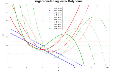
Die zugeordneten (verallgemeinerten) Laguerre-Polynome hängen mit den gewöhnlichen Laguerre-Polynomen über

zusammen. Ihre Rodrigues-Formel lautet

Die zugeordneten Laguerre-Polynome erfüllen die zugeordnete Laguerre-Gleichung

Die ersten zugeordneten Laguerre-Polynome lauten:


![L_{2}^{k}(x)={\frac {1}{2}}\,\left[x^{2}-2\,(k+2)\,x+(k+1)(k+2)\right]](/svg/ae15ad7b67ff44bbd7e3003468ef214b46a99f37.svg)
![{\displaystyle L_{3}^{k}(x)={\frac {1}{6}}\,\left[-x^{3}+3\,(k+3)\,x^{2}-3\,(k+2)\,(k+3)\,x+(k+1)\,(k+2)\,(k+3)\right]}](/svg/3908ce0eabd5a11f1e577eff87d3829369bfddc5.svg)
Zur Berechnung lässt sich die Rekursionsformel

verwenden.
Der Sturm-Liouville-Operator lautet

und mit der Gewichtsfunktion
gilt:


Zugeordnete Laguerre-Polynome lassen sich als Wegintegrale ausdrücken:

Dabei ist  ein Weg, der den Ursprung einmal im Gegenuhrzeigersinn umrundet und die
wesentliche Singularität bei 1 nicht einschließt.
ein Weg, der den Ursprung einmal im Gegenuhrzeigersinn umrundet und die
wesentliche Singularität bei 1 nicht einschließt.
Wasserstoffatom
Die Laguerre-Polynome haben eine Anwendung in der Quantenmechanik bei der Lösung der Schrödinger-Gleichung für das Wasserstoffatom bzw. im allgemeinen Fall für ein Coulomb-Potential. Mittels der zugeordneten Laguerre-Polynome lässt sich der Radialanteil der Wellenfunktion schreiben als

(Normierungskonstante  ,
charakteristische Länge
,
charakteristische Länge  ,
Hauptquantenzahl ,
Bahndrehimpulsquantenzahl
,
Hauptquantenzahl ,
Bahndrehimpulsquantenzahl  ).
Die zugeordneten Laguerre-Polynome haben hier also eine entscheidende Rolle. Die
normierte Gesamtwellenfunktion ist durch
).
Die zugeordneten Laguerre-Polynome haben hier also eine entscheidende Rolle. Die
normierte Gesamtwellenfunktion ist durch
![{\displaystyle \Psi _{n,l,m}(r,\vartheta ,\varphi )={\sqrt {\frac {4\,(n-l-1)!}{(n+l)!\;n\,(na_{0}/Z)^{3}}}}\left[{\frac {2r}{na_{0}/Z}}\right]^{l}\exp {\left\{-{\frac {r}{na_{0}/Z}}\right\}}\;L_{n-l-1}^{2l+1}\left({\frac {2r}{na_{0}/Z}}\right)\;Y_{l,m}(\vartheta ,\varphi )}](/svg/45c656de94c4f217677df1ae610d165293d61938.svg)
gegeben, mit der Hauptquantenzahl
,
der Bahndrehimpulsquantenzahl
,
der magnetischen Quantenzahl
 ,
dem bohrschen
Radius
,
dem bohrschen
Radius  und der Kernladungszahl
 .
Die Funktionen
.
Die Funktionen  sind die zugeordneten Laguerre-Polynome,
  die Kugelflächenfunktionen.
Anmerkungen
- ↑
Wegen der linearen Parametrisierung kann o.B.d.A.
das Differential
 gewählt werden.
 - ↑ In der Physik wird statt beschränkt üblicherweise der Begriff normiert verwendet.


© biancahoegel.de
Datum der letzten Änderung: Jena, den: 25.03. 2021