Airy-Funktion
Die Airy-Funktion  bezeichnet eine spezielle
Funktion in der Mathematik. Die Funktion
und die verwandte Funktion
bezeichnet eine spezielle
Funktion in der Mathematik. Die Funktion
und die verwandte Funktion  ,
die ebenfalls Airy-Funktion genannt wird, sind Lösungen der linearen
Differentialgleichung
,
die ebenfalls Airy-Funktion genannt wird, sind Lösungen der linearen
Differentialgleichung

auch bekannt als Airy-Gleichung. Sie beschreibt unter anderem die Lösung der Schrödinger-Gleichung für einen linearen Potentialtopf.
Die Airy-Funktion ist nach dem britischen Astronomen George Biddell Airy
benannt, der diese Funktion in seinen Arbeiten in der Optik
verwendete (Airy 1838). Die Bezeichnung
wurde von Harold
Jeffreys eingeführt.
Definition
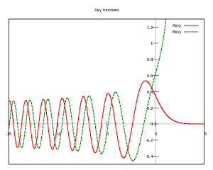
Für reelle Werte  ist die Airy-Funktion als Parameterintegral
definiert:
ist die Airy-Funktion als Parameterintegral
definiert:

Eine zweite, linear unabhängige Lösung der Differentialgleichung ist die
Airy-Funktion zweiter Art  :
:

Eigenschaften
Asymptotisches Verhalten
Für
gegen  lassen sich
  und
und  mit Hilfe der WKB-Näherung
approximieren:
mit Hilfe der WKB-Näherung
approximieren:

Für
gegen  gelten die Beziehungen:

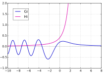
Nullstellen
Die Airy-Funktionen haben nur Nullstellen auf der negativen reellen
Achse.
Die ungefähre Lage folgt aus dem asymptotischen Verhalten für  zu
zu


Spezielle Werte
Die Airy-Funktionen und ihre Ableitungen haben für  die folgenden Werte:
![{\displaystyle {\begin{aligned}\mathrm {Ai} (0)&{}={\frac {1}{{\sqrt[{3}]{9}}\cdot \Gamma ({\frac {2}{3}})}},&\quad \mathrm {Ai} '(0)&{}=-{\frac {1}{{\sqrt[{3}]{3}}\cdot \Gamma ({\frac {1}{3}})}},\\\mathrm {Bi} (0)&{}={\frac {1}{{\sqrt[{6}]{3}}\cdot \Gamma ({\frac {2}{3}})}},&\quad \mathrm {Bi} '(0)&{}={\frac {\sqrt[{6}]{3}}{\Gamma ({\frac {1}{3}})}}.\end{aligned}}}](/svg/a85175b026a300ea1e494ba99b326df0e329f29f.svg)
Hierbei bezeichnet  die Gammafunktion. Es folgt,
dass die Wronski-Determinante
von
und
gleich
die Gammafunktion. Es folgt,
dass die Wronski-Determinante
von
und
gleich  ist.
ist.
Fourier-Transformierte
Direkt aus der Definition der Airy-Funktion
(siehe oben) folgt deren Fourier-Transformierte.

Man beachte die hier verwendete symmetrische Variante der Fourier-Transformation.
Weitere Darstellungen
- Unter Verwendung der hypergeometrischen
Funktion


- Für
 lassen sie sich auch mit der modifizierten
Bessel-Funktion erster Art
lassen sie sich auch mit der modifizierten
Bessel-Funktion erster Art  so darstellen:
![{\displaystyle \mathrm {Ai} (x)={\frac {1}{3}}{\sqrt {x}}\left[I_{-1/3}\left({\frac {2}{3}}x^{3/2}\right)-I_{1/3}\left({\frac {2}{3}}x^{3/2}\right)\right]}](/svg/b1f0cd33e711461cb3ab410a2d4b0af8dcb99aca.svg)
![{\displaystyle \mathrm {Bi} (x)={\sqrt {\frac {x}{3}}}\left[I_{-1/3}\left({\frac {2}{3}}x^{3/2}\right)+I_{1/3}\left({\frac {2}{3}}x^{3/2}\right)\right]}](/svg/9175279c9f086c7d1242484b4430f327531ed036.svg)
- Eine andere unendliche Integraldarstellung für
 lautet

- Es gibt die Reihendarstellungen


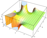
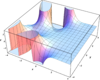
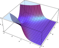
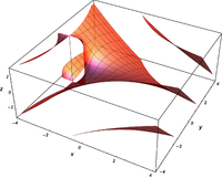
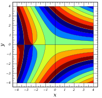
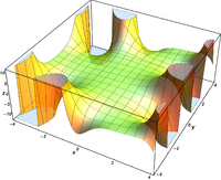
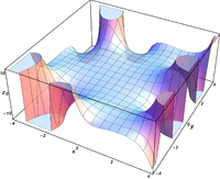
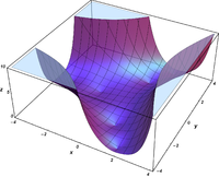
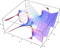
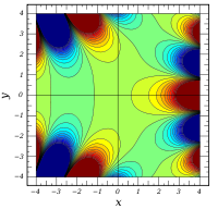
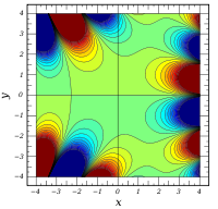
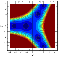
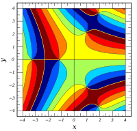
Komplexe Argumente
und
sind ganze
Funktionen. Sie lassen sich also auf der gesamten komplexen Ebene analytisch
fortsetzen.
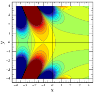
![{\displaystyle \Re \left[\mathrm {Ai} (x+iy)\right]}](/svg/505e2f06e2e8d14027c46f1f4b1ac72367f85b58.svg)
|
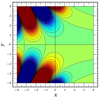
![{\displaystyle \Im \left[\mathrm {Ai} (x+iy)\right]}](/svg/6c4ca8fdfe9c79b62f9becbb2687b12f68d42e18.svg)
|

|
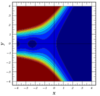
![{\displaystyle \mathrm {arg} \left[\mathrm {Ai} (x+iy)\right]\,}](/svg/190234ee42ad7ac3a352d501c46e3bfcb4e64be4.svg)
|
|---|---|---|---|
 |
 |
 |
 |
 |
 |
 |
 |
![{\displaystyle \Re \left[\mathrm {Bi} (x+iy)\right]}](/svg/3a86d49867d1f711cbe25936ea7982c44f005c53.svg)
|
![{\displaystyle \Im \left[\mathrm {Bi} (x+iy)\right]}](/svg/b658626fb2e88ae1d2a3ff37af457b29b0f17e0d.svg)
|

|
![{\displaystyle \mathrm {arg} \left[\mathrm {Bi} (x+iy)\right]\,}](/svg/1e6398901714ff29a82ca26b13f90f473377a731.svg)
|
|---|---|---|---|
 |
 |
 |
 |
 |
 |
 |
 |
Verwandte Funktionen
Airy-Zeta-Funktion
Zu der Airy-Funktion lässt sich analog zu den anderen Zeta-Funktionen die Airysche Zeta-Funktion definieren als

wobei die Summe über die reellen (negativen) Nullstellen von
geht.
Scorersche Funktionen
 und
und  .
.Manchmal werden auch die beiden weiteren Funktionen
und
zu den Airy-Funktionen dazugerechnet. Die Integral-Definitionen lauten


Sie lassen sich auch durch die Funktionen
und
darstellen.


© biancahoegel.de
Datum der letzten Änderung: Jena, den: 20.12. 2021