Exakte Differentialgleichung
ΦEine exakte (oder vollständige) Differentialgleichung ist eine gewöhnliche Differentialgleichung der Form
 ,
,
bei der es eine stetig
differenzierbare Funktion  gibt, so dass gilt
 und
und  .
.
Eine solche Funktion  heißt dann Potentialfunktion des Vektorfelds
 .
.
Einführung
Die Differentialgleichung  wird durch die Trennung
der Variablen gerne in der Darstellung
wird durch die Trennung
der Variablen gerne in der Darstellung
angegeben. Der Vorteil dieser Darstellung liegt darin begründet, dass die
linke Seite der Differentialgleichung – also  – als Bestandteil eines totalen
Differentials aufgefasst werden kann, mit
– als Bestandteil eines totalen
Differentials aufgefasst werden kann, mit
 .
.
Hierbei übernimmt die Funktion
die Bedeutung eines Skalarpotentials
mit der Bedingung  sowie
sowie  .
Demnach muss es ein Vektorfeld
geben, welches aus dem Gradienten des Skalarpotentials gebildet werden kann,
also
.
Demnach muss es ein Vektorfeld
geben, welches aus dem Gradienten des Skalarpotentials gebildet werden kann,
also
 .
.
Sind  und
und  stetig partiell
differenzierbar und ist der Definitionsbereich von
und
ein einfach zusammenhängendes
Gebiet
stetig partiell
differenzierbar und ist der Definitionsbereich von
und
ein einfach zusammenhängendes
Gebiet  ,
so gibt es genau dann ein Skalarpotential
,
wenn die sogenannte Integrabilitätsbedingung
,
so gibt es genau dann ein Skalarpotential
,
wenn die sogenannte Integrabilitätsbedingung

erfüllt ist. Demzufolge muss für die zweifach stetig partiell
differenzierbare Funktion
gelten:
 .
.
Der Sachverhalt, dass  ist, wird im Satz
von Schwarz behandelt. Zudem bedeutet die angegebene
Integrabilitätsbedingung auch, dass wenn die Rotation
des Vektorfeldes
auf einem einfach zusammenhängenden Gebiet verschwindet, also
ist, wird im Satz
von Schwarz behandelt. Zudem bedeutet die angegebene
Integrabilitätsbedingung auch, dass wenn die Rotation
des Vektorfeldes
auf einem einfach zusammenhängenden Gebiet verschwindet, also  gilt, ein Skalarpotential
existiert.
gilt, ein Skalarpotential
existiert.
Wird andererseits die rechte Seite der Differentialgleichung  mit dem totalen
Differential der Funktion
verknüpft, so ergibt sich eine Pfaffsche
Form in der Darstellung
mit dem totalen
Differential der Funktion
verknüpft, so ergibt sich eine Pfaffsche
Form in der Darstellung  und nach einer beidseitigen Integration der Gleichung folgt
 .
.
Somit wird anschaulich, dass es eine Konstante  geben muss, die für alle
  die Funktion
erfüllt. Die Lösung
die Funktion
erfüllt. Die Lösung  ist daher die Anfangsbedingung der Differentialgleichung und stellt eine Äquipotentiallinie
dar.
ist daher die Anfangsbedingung der Differentialgleichung und stellt eine Äquipotentiallinie
dar.
wird im Zusammenhang mit der exakten Differentialgleichung auch als Erstes Integral bezeichnet.
Definition
In einem einfach zusammenhängenden Gebiet
ist eine exakte Differentialgleichung gegeben durch

wenn folgende Voraussetzungen gelten:
- Die Funktionen
 sind stetig partiell differenzierbar.
- Die Integrabilitätsbedingung
 ist erfüllt.
- Es existiert ein zweifach stetig partiell differenzierbares
Skalarpotential ,
so dass
sowie
gilt.
- Es ist ein Anfangswert
 vorgegeben.
Lösungsmethode
Um die exakte Differentialgleichung zu lösen, ist es erforderlich, das Skalarpotential
wie folgt zu ermitteln :
- Integrabilitätsbedingung: Die Differentialgleichung ist exakt, wenn die Integrabilitätsbedingung

- erfüllt ist. Falls dies nicht der Fall ist, kann die Differentialgleichung eventuell mittels eines integrierenden Faktors gelöst werden.
- Erstes Integral: Wenn eine exakte Differentialgleichung vorliegt, wird mittels Integration aus der Beziehung
- das Skalarpotential zu

- bestimmt. Dabei ist
 eine von
  unabhängige Integrationskonstante, die jedoch bzgl.
  variabel ist. Insofern ist das Skalarpotential bis auf eine unbekannte
Funktion
bestimmt. Um nun die noch unbekannte Funktion
zu ermitteln, wird die Integrabilitätsbedingung in der Integraldarstellung
genutzt. Durch Integration von
variabel ist. Insofern ist das Skalarpotential bis auf eine unbekannte
Funktion
bestimmt. Um nun die noch unbekannte Funktion
zu ermitteln, wird die Integrabilitätsbedingung in der Integraldarstellung
genutzt. Durch Integration von - erhält man

- wobei die rechte Seite der Gleichung
 liefert. Nach Umformen folgt
- Durch nochmalige Integration ergibt sich

- und somit lautet eine Lösung des gesuchten Skalarpotentials

- Die Stammfunktion
wird auch als Erstes Integral der exakten Differentialgleichung
bezeichnet.
- Anfangsbedingung: Bei allen zuvor durchgeführten Integrationen
blieb die Integrationskonstante unberücksichtigt, da diese aus dem Anfangswert
berechnet wird. Da neben der exakten Differentialgleichung für die Lösung ein
Anfangswert nötig ist, kann nun mit
das Skalarpotential
ermittelt werden.
-
- Ohne Anfangswert: Ist der Anfangswert
 nicht bekannt, so ergibt die Differentialgleichung
  die Lösung .
Diese Anfangsbedingung liefert dann, eingesetzt in das Erste Integral, die
gewünschte Lösung der exakten Differentialgleichung
die Lösung .
Diese Anfangsbedingung liefert dann, eingesetzt in das Erste Integral, die
gewünschte Lösung der exakten Differentialgleichung
- Ohne Anfangswert: Ist der Anfangswert

-
- Mit Anfangswert: Ist ein Anfangswert
vorgegeben, so muss die Gleichung
 erfüllt sein. Dieser Anfangswert liefert dann, eingesetzt in das Erste
Integral, die gewünschte Lösung der exakten Differentialgleichung
erfüllt sein. Dieser Anfangswert liefert dann, eingesetzt in das Erste
Integral, die gewünschte Lösung der exakten Differentialgleichung
- Mit Anfangswert: Ist ein Anfangswert

- einfach zusammenhängendes Gebiet: Schlussendlich ist zu prüfen, ob die Lösung ein einfach zusammenhängendes Gebiet abdeckt. Falls dies nicht der Fall ist, muss geprüft werden, ob durch geeignete Restriktionen die Lösung auf ein einfach zusammenhängendes Gebiet reduziert werden kann.
- Beispiel
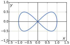

Es soll die exakte Differentialgleichung der Lemniskate von Gerono berechnet werden. Es wird also die Differentialgleichung

mit dem Anfangswert  betrachtet. Demnach ist

und die Integrabilitätsbedingung ergibt
 .
.
Die Differentialgleichung ist also exakt und das Erste Integral kann sofort
bestimmt werden. Dazu wird zunächst
berechnet

Somit ist  und das zweite Integral verschwindet, da der Integrand nicht von
abhängig ist. Die Integrationskonstanten werden, wie zuvor ausgeführt, nicht
berücksichtigt. Unter dieser Voraussetzung lässt sich das Erste Integral
bestimmen zu
und das zweite Integral verschwindet, da der Integrand nicht von
abhängig ist. Die Integrationskonstanten werden, wie zuvor ausgeführt, nicht
berücksichtigt. Unter dieser Voraussetzung lässt sich das Erste Integral
bestimmen zu

Mit  und dem Anfangswert
ergibt sich als Lösung der impliziten
Kurve
und dem Anfangswert
ergibt sich als Lösung der impliziten
Kurve
- .
Integrierende Faktoren
Für eine gewöhnliche Differentialgleichung der Form  ,
welche die Integrabilitätsbedingung
,
welche die Integrabilitätsbedingung  nicht erfüllt, lässt sich gelegentlich eine nullstellenfreie stetig
differenzierbare Funktion
nicht erfüllt, lässt sich gelegentlich eine nullstellenfreie stetig
differenzierbare Funktion  derart bestimmen, dass

eine exakte Differentialgleichung wird. In diesem Fall wird  als integrierender Faktor oder eulerscher Multiplikator
bezeichnet. Da
nach Definition niemals Null wird, hat die exakte Differentialgleichung
dieselben Lösungen wie vor der Multiplikation mit
als integrierender Faktor oder eulerscher Multiplikator
bezeichnet. Da
nach Definition niemals Null wird, hat die exakte Differentialgleichung
dieselben Lösungen wie vor der Multiplikation mit  Dabei ist
  genau dann ein integrierender Faktor, wenn die Integrabilitätsbedingung in der
Darstellung
genau dann ein integrierender Faktor, wenn die Integrabilitätsbedingung in der
Darstellung

erfüllt wird.
Es ist normalerweise schwierig, diese partielle Differentialgleichung
allgemein zu lösen. Da man aber nur eine spezielle Lösung
benötigt, wird man versuchen, mit speziellen Ansätzen für
eine Lösung zu finden. Solche Ansätze könnten beispielsweise lauten:
 .
.
Integrierender Faktor  und
und 
Ein einfaches Beispiel für einen integrierenden Faktor
ist dann gegeben, wenn dieser nur von einer Variablen
oder
abhängt.
Zunächst wird der Fall betrachtet bei dem der integrierende Faktor nur von
abhängig ist und infolge dessen  ist. Unter dieser Voraussetzung ergibt die Integrabilitätsbedingung
im Zusammenhang mit der Produktregel folgende Darstellung

und nach Umformen folgt

was sich auch schreiben lässt als

Die Kettenregel für die logarithmische Ableitung liefert schließlich

Beidseitige Integration dieser Gleichung ergibt unter Auslassung der Integrationskonstanten

oder

Demnach ist der integrierende Faktor
nur von
abhängig, wenn folgender Ausdruck nur eine Funktion von
ist:

Auf die gleiche Weise lässt sich zeigen, dass der integrierende Faktor
nur von
abhängt, wenn

nur eine -Abhängigkeit
hat und der integrierende Faktor lautet dann

- Beispiel
Ausgehend von der Differentialgleichung

mit

und

wird erkennbar, dass die Integrabilitätsbedingung nicht erfüllt ist. Da
nur von
abhängt, ist es sinnvoll den integrierenden Faktor so zu wählen, dass
nur von
abhängig ist und somit

Also lautet der integrierende Faktor

Integrierender Faktor 
Hängt  von
von  ab, so lautet der integrierende Faktor

- Beweis
Es ist

und auf die gleiche Weise ergibt sich

Wird nun die Integrabilitätsbedingung in die Darstellung  gebracht, so folgt

Literatur
- Harro Heuser: Gewöhnliche Differentialgleichungen, Vieweg+Teubner 2009 (6. Auflage), Seite 91–102, ISBN 978-3-8348-0705-2


© biancahoegel.de
Datum der letzten Änderung: Jena, den: 18.06. 2021